
Data prep to deployment: Maximizing generative AI value with ClearScape Analytics™ in the cloud
Explore an end-to-end generative AI pipeline that illustrates the usage of different tools in the VantageCloud ecosystem.
ClearScape Analytics, the powerful analytics engine in Teradata VantageCloud that enables enterprises to seamlessly deploy end-to-end AI/ML pipelines, offers considerable value for organizations looking to reap the benefits of generative AI. ClearScape Analytics streamlines each step of the machine learning (ML) lifecycle, including understanding and defining the problem, preprocessing relevant data, model training, model deployment, and model operations.
In this post, we’ll explore an end-to-end generative AI pipeline to illustrate the usage of different tools in the VantageCloud ecosystem to easily define a problem; collect, clean, and preprocess data; integrate training data to cloud-native ML tools; and operationalize the trained model. The initial steps, problem definition, data exploration, and data preparation are covered with relevant code snippets that can be replicated. Starting from the training step, the process is detailed in a descriptive fashion, making it easy to follow along, and the required VantageCloud instance is provided through ClearScape Analytics Experience, a free, self-service demo environment that allows you to explore over 80+ real-world use cases across multiple industries and analytic functions within a fully functional VantageCloud environment.
Requirements
To follow along with this post, you’ll need a ClearScape Analytics Experience environment. You can provision your free, self-service demo environment in minutes.
Table of contents
- Problem definition
- Loading of sample data
- Data exploration
- Data preprocessing
- Model training
- Model operationalization
Problem definition
An online retailer is planning to develop a recommendation system. This system aims to predict the subsequent product a customer will add to their online shopping cart, offering pertinent recommendations associated with marketing initiatives, seasonal promotions, and so on. Models that use natural language processing (NLP) excel at tasks like these. NLP models can predict the subsequent word in a sentence when given only a segment of the sentence. Systems such as OpenAI’s ChatGPT largely operate on this principle.
When viewing the shopping cart scenario through this lens, we can liken the shopping cart to a sentence, with each product added to the cart serving as a “word” in that “sentence.” Previous orders function as the context on which the model can train until it can make informed predictions. As the model trains, it unravels the inherent connections between “products” in an order, which empowers it to make accurate forecasts.
To achieve the business purpose described, we need to explore the available data, preprocess it, make the preprocessed data available for training, train an NLP model, and deploy and monitor the resulting model. For purposes of the illustrative scenario, we will initiate by loading some data into a Teradata VantageCloud instance.
Loading of sample data
Environment setting
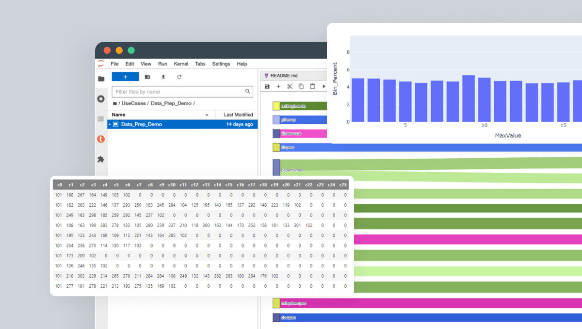
We will be interacting with the Teradata VantageCloud instance through a ClearScape Analytics Experience Jupyter Notebook. Follow the steps below:
Create a ClearScape Analytics Experience account.
1. Create an environment.
2. Select Run Demos Using Jupyter.
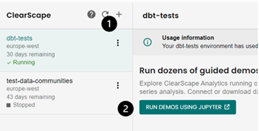
Creating a ClearScape Analytics Experience environment
3. Navigate to the Use Cases folder.
4. Create a new folder with a name of your choice.
5. Create a new Jupyter Python Notebook with a name of your choice inside the folder.
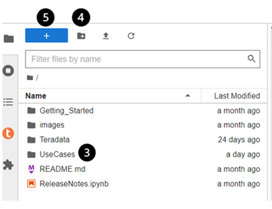
Creating a Jupyter Notebook
Loading of data
Import the Teradata ML libraries into the notebook.
import teradataml as tdml
import json

import pandas as pd

import seaborn as sns

import plotly.express as px

import tdnpathviz
Create a database session in your Jupyter Notebook.
%run -i ../startup.ipynb

eng = tdml.create_context(host = 'host.docker.internal', username='demo_user', password = password)
At this step, we will not define any database in the context. Creating the default database will be the first query we run.
The connection will request a password. This is the password you used while creating your ClearScape Analytics Experience environment.
We run the following commands in our notebook to create the default database.
qry = """

CREATE DATABASE teddy_retailers_ml

AS PERMANENT = 110e6;

"""

tdml.execute_sql(qry)
Once the default database is created, we execute the `create_context` command again to set the default database. This simplifies all further queries.
eng = tdml.create_context(host = 'host.docker.internal', username='demo_user', password = password, database = 'teddy_retailers_ml')
With the database created and defined as default, we can proceed to run the queries that load the data into the database. For this, we leverage the connection we have created.
qry='''

CREATE MULTISET TABLE teddy_retailers_ml.products AS

(

 SELECT product_id, product_name, department_id

  FROM (

 LOCATION='/gs/storage.googleapis.com/clearscape_analytics_demo_data/DEMO_groceryML/products.csv') as products

) WITH DATA;

'''

tdml.execute_sql(qry)


qry='''

CREATE MULTISET TABLE teddy_retailers_ml.order_products AS

(

 SELECT order_id, product_id, add_cart_order

  FROM (

 LOCATION='/gs/storage.googleapis.com/clearscape_analytics_demo_data/DEMO_groceryML/order_products.csv') as orders_products

) WITH DATA;

'''

tdml.execute_sql(qry)
With the data loaded into the database, we can explore the data.
Data exploration
We have two datasets imported into the database as tables. The table `products` contains general product information, `product_id`, `product_name`, and `department_id`. This table is mainly used to retrieve product names to illustrate examples in the data exploration stage. The `order_products` table contains the records of orders, identified with their specific IDs, detailing the products — `product_id` — added to each order and the sequence — `add_cart_order` — in which they were added to the cart. This table is central to our analysis.
We can analyze the data in the `orders_products` table by importing it into a Teradata DataFrame using the command provided below:
orders = tdml.DataFrame("order_products")

orders
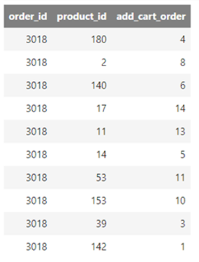
Products as they are added to orders in the dataset
The example shows a list of products added to order number 3018. The first product added to that order, in this example, is the product with the ID 142, while the first one that appears listed, 180, corresponds to the fourth item added to the cart.
Records shown depend on how the DataFrame is indexed and paginated for display.
A typical analysis in this context involves determining the distribution of the number of products added to each order. This insight helps establish an appropriate baseline for the average length of the “sentences” (orders) that we will utilize for making predictions.
We group the `order_product` data by `order_id` and aggregate on the count of `product_id`:
counts_per_order = orders.groupby("order_id").agg({"product_id": "count"})

counts_per_order
From this, we obtain a DataFrame that describes the number of products added to each order.
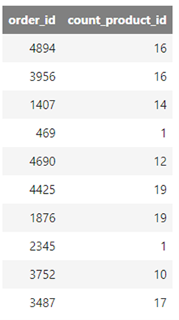
Number of products in each order
We can apply the `teradataml` histogram function to this table to create a DataFrame suited for histogram visualization. To generate a visual representation using a plotting library, we arrange the resulting DataFrame by `Label` and transform it into a standard pandas DataFrame.
In the resulting DataFrame, every row stands for a bin in the histogram, defining a range where data points are collected. It includes the label for the bin, the number of data points within that specific range, the percentage of that count in relation to the total data points, and the minimum and maximum limits of each bin. For more details, explore the ML histogram documentation in the Teradata Developer Portal.
count_prod_hist = tdml.Histogram(data=counts_per_order,

    target_columns="count_product_id",

    method_type="Sturges")

count_prod_hist_pd = count_prod_hist.result.sort("Label").to_pandas()

count_prod_hist_pd
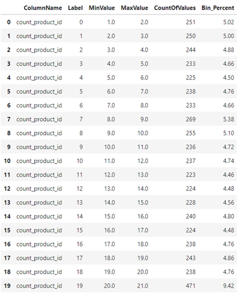
Histogram table suitable for generating a histogram visualization
To construct the plot, we use the histogram DataFrame as the data source, designating the maximum value of products added to the order as the X-axis and the percentage of products in that specific bin as the Y-axis. In the resulting graph, we can see that most of the orders, north of 9% (X-axis), contain more than 20 products (Y-axis).
fig = px.bar(count_prod_hist_pd, x="MaxValue", y="Bin_Percent")

fig.show()

Histogram showing the maximum number of products per order in the dataset
Since we’re operating with a simulated dataset, the distribution may not reflect typical trends, but we’ll proceed with it.
Another standard exploratory step involves identifying the most popular products and the most frequent sequences in which these products are added to the shopping cart.
To achieve this, we need to bring the `products` table to a corresponding Teradata DataFrame.
products = tdml.DataFrame('products')

products
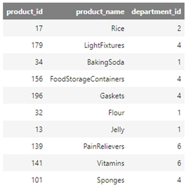
Product information table
We can merge the two DataFrame structures — `orders` and `products`, based on the product ID. This enables accessing product details from the orders DataFrame. Prefixes are needed to disambiguate between similarly named columns.
orders_products_merged = orders.join(

  other = products,

  on = "product_id",

  how = "inner",

  lsuffix = "ordrs",

  rsuffix = "prdt")

orders_products_merged
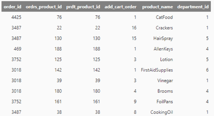
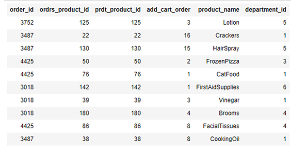
Product information table added to order data
In this DataFrame, we can examine the products most frequently ordered. We do this by grouping based on `product_name`, tallying the count of `orders_product_id`, and then sorting these results in descending order.
product_counts = orders_products_merged.groupby('product_name').agg({"ordrs_product_id": "count"})

product_counts.sort("count_ordrs_product_id", ascending=False)
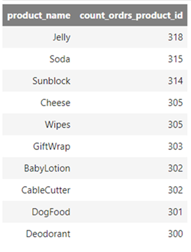
Most ordered products in the dataset
To identify the most common sequences in which products are added to the shopping cart, we must identify the sequences in which products were included in each of the orders. For ease of analysis, we’ll express these sequences as pairs. This implies we’ll identify pairs of products in which one product frequently follows another.
The Teradata nPath® function is routinely used for such purposes. This function is particularly useful for identifying sequential patterns within data. The primary inputs for nPath are the rows to be analyzed, the column used for data partitioning, and the column that dictates the order of the sequence.
In our case, we’ll perform the path analysis on the data in `orders_products_merged`. Since we aim to identify sequential patterns in relation to orders, our partition column is `order_id`. Given that we want to construct the sequence based on the order in which products were added to the cart, our ordinal column is `add_cart_order`.
Other key components of the nPath function include the conditions that a data point should meet to be included in the sequence and the patterns we’re identifying among the rows that meet the condition. These are supplied to nPath as the parameters `symbol` and `pattern`, respectively.
The nPath function for our purpose would be as follows:
common_seqs = tdml.NPath(

    data1=orders_products_merged,

    data1_partition_column="order_id",

    data1_order_column="add_cart_order",

    mode="OVERLAPPING",

    pattern="A.A",

    symbols="TRUE as A",

    result=[

        "FIRST (order_id OF A) AS order_id",

        "ACCUMULATE (product_name OF A) AS path",

        "COUNT (* OF A) AS countrank"

        ]

    ).result
The symbol `A` merely implies that a `product_id` `A` exists in an order, thus `True as A`. The pattern `A.A` is fulfilled each time a given product `A`, follows another product `A` added previously to the shopping cart. We set the mode as overlapping, since the second element of a given pair could be the first element of another pair.
The `FIRST` function retrieves the `order_id` from the initial row that matched the pattern, while ACCUMULATE constructs the path with the `product_name` found in every matched row, following the sequence defined by `add_cart_order`.
To obtain a count of the most common pairs, we group by `path` and aggregate by the count of `order_id`, sorting the results in descending order based on the count.
common_seqs.groupby('path').agg({"order_id": "count"}).sort('count_order_id',ascending=False)
The most frequently ordered pairs are listed below. It’s important to note that the data is simulated, hence the patterns observed:
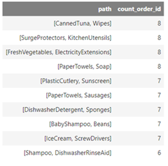
Graphic visualization of product pairs
We can visualize the paths by importing the `plot_first_main_paths` graph from the Teradata tdnpathviz package:
from tdnpathviz.visualizations import plot_first_main_paths

plot_first_main_paths(common_seqs,path_column='path',id_column='order_id')
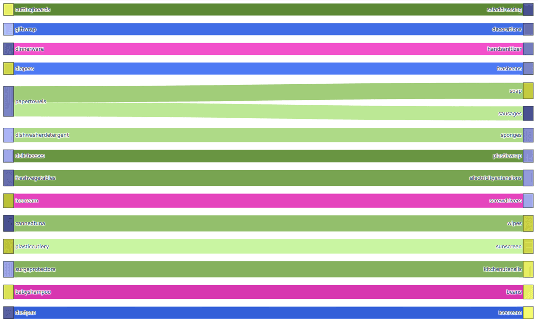
Path visualization regarding product pairs added to orders. Only main paths are shown.
Data preprocessing
NLP models like BERT are developed using extensive text corpora. To facilitate their training, these models translate words in languages such as English into a series of tokens, which are sequential identifiers. The essence of the training process involves the model learning to predict a specific token based on its surrounding context. This technique has proven to be an effective way for computer systems to predict and generate language.
In attempting to predict the next product a customer will add to their shopping cart, we employ a method analogous to training language models. In this case, our training corpus is comprised of previous orders within our system or our `order_products` data. Each product within an order is to be substituted by its corresponding token, a sequential identifier.
As we previously did during the data exploration phase, we will transform each order into an ordered sequence of products, but this time we’ll construct the sequence using sequential identifiers, or tokens, rather than product names. Additionally, we’ll incorporate markers to indicate the beginning and end of each order. This specially formatted data is then passed to the training stage. Here, the model will derive a probability distribution predicting the likelihood of a particular product being added to the shopping cart, based on the products that have been added previously.
To prepare the data for processing, by an ML library or a pre-trained model, especially those required for generative AI through NLP, we need to verify a few things:
Product identifiers must be sequential. This ensures that the NLP model can process them as it would with words in a sentence.
Just as we use a capital letter to start a sentence and a period to end it in English grammar, our order sequences (analogous to “sentences” in this context) also need specific markers to denote the beginning and end of each sequence.
We must eliminate null values. ML training via NLP tools fundamentally involves matrix multiplication, which can only be performed with numerical values.
Adding sequential product identifiers
In our specific dataset, the product identifier `product_id` happens to be sequential. However, this is just a matter of chance, not design. For this reason, we’ll assume that the `product_id` is not sequential. This allows us to define the starting point of the sequence, which we can utilize to define our “sentence” start and “sentence” end markers.
We’ll define the number `101` as our “sentence” start marker and the number `102` as our “sentence” end marker. With these two constants defined, we can assign a sequential identifier to the items in our `products` table. This sequential identifier will start at `103` and continue from there.
We create a volatile table `temp` that matches each product `product_id` with the sequential identifier that we are creating. For this, we use SQL’s `ROW_NUMBER` and `OVER` statements. This table will have a primary index on `product_id` we want this table to be preserved with the session, so we define the parameter `ON_COMMIT_PRESERVE_ROWS`:
create_table_qry = '''

CREATE VOLATILE TABLE temp AS (

    SELECT product_id,

   ROW_NUMBER() OVER (ORDER BY product_id) + 102 as seq_product_id

    FROM products

) WITH DATA PRIMARY INDEX (product_id) ON COMMIT PRESERVE ROWS;

'''

tdml.execute_sql(create_table_qry)
To create the sequential `product_id`, this statement retrieves the row number of each record in the `products` table, ordered by `product_id`, and adds 102 to that number. The result is defined as `seq_product_id`.
We create a new column in our `products` table to store the sequential product identifiers:
add_column_qry = '''

ALTER TABLE products

ADD seq_product_id INTEGER;

'''

tdml.execute_sql(add_column_qry)
Finally, we add the sequential identifiers to our product’s table, as `seq_product_id`:
modify_table_qry = '''

UPDATE products

SET seq_product_id = (

    SELECT temp.seq_product_id

    FROM temp

    WHERE products.product_id = temp.product_id

);

'''

tdml.execute_sql(modify_table_qry)
The resulting table can be ingested again into our `products` DataFrame.
products = tdml.DataFrame('products')

products.sort('seq_product_id')
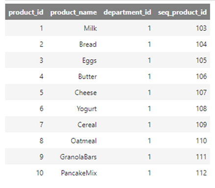
Product information data with added sequential identifiers
Order tokenization
As mentioned, we’ll create sequences of products added per order as we did during the data exploration phase. However, we’ll use the sequential identifiers we recently produced rather than product names in the `path`. These sequential identifiers serve as tokens to identify the products. We’ll also add markers for the beginning and end of the “sequence” — order, in our case.
First, we must recreate the `orders_products_merged` DataFrame, this time with the updated `products` DataFrame in the join. We keep all the columns on the `products` DataFrame for reference and simplicity. In a real scenario, we would keep only the IDs.
orders_products_merged = orders.join(

    other = products,

    on = "product_id",

    how = "inner",

    lsuffix = "ordrs",

   rsuffix = "prdt")

orders_products_merged
Product information data added to orders data
From this modified `orders_products_merged`, we’ll generate a preliminary DataFrame with the orders represented as sequences of products.
At this stage, each record will have at least two items. If only one item was added to the shopping cart, for example, the record would be populated with the beginning-of-sentence marker and the sequential identifier of the product added. To achieve this, we’ll add a new column to the `orders_products_merged` DataFrame with the constant value `101`, which is our beginning-of-sentence marker.
orders_products_merged = orders_products_merged.assign(

    bgn = 101

).select(["order_id", "add_cart_order", "seq_product_id", "bgn"])

orders_products_merged
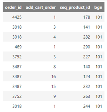
Beginning of sentence marker added to orders data
With this updated DataFrame, we’ll use Teradata’s nPath function to generate the sequences of products per order. This process resembles what we did in the data exploration stage. The difference here is that we won’t include the `order_id`, as it is not part of the “sentence” and is not relevant for training a model. Also, we won’t accumulate all tokens in one column; instead, we’ll have a distinct column for each token.
Additionally, the pattern will not look for matches on product pairs; we’ll add any sequence, even if it only contains one product. For this, we’ll use the wildcard `*`.
During our data exploration, we uncovered a crucial piece of information that is beneficial now: the maximum number of products in an order in our dataset is `21`. At this stage, we must allocate a column for each token. We intend to streamline column creation by only adding them where tokens exist.
Additionally, we must allocate at least one extra column to accommodate an end-of-sentence marker for longer lists. Given that 25 is a reasonably round figure, we will incorporate 25 columns into the dataset we’re preparing.
Carrying out all the processes above is made significantly easier with Teradata’s nPath function.
prepared_ds = tdml.NPath(

    data1=orders_products_merged,

    data1_partition_column="order_id",

    data1_order_column="add_cart_order",

    mode="NONOVERLAPPING",

    pattern="A*",

    symbols="TRUE as A",

    result=["FIRST (bgn OF A) AS c0",

            "NTH (seq_product_id, 1 OF A) as c1",

            "NTH (seq_product_id, 2 OF A) as c2",

            "NTH (seq_product_id, 3 OF A) as c3",

            "NTH (seq_product_id, 4 OF A) as c4",

            "NTH (seq_product_id, 5 OF A) as c5",

            "NTH (seq_product_id, 6 OF A) as c6",

            "NTH (seq_product_id, 7 OF A) as c7",

            "NTH (seq_product_id, 8 OF A) as c8",

            "NTH (seq_product_id, 9 OF A) as c9",

            "NTH (seq_product_id, 10 OF A) as c10",

            "NTH (seq_product_id, 11 OF A) as c11",

            "NTH (seq_product_id, 12 OF A) as c12",

            "NTH (seq_product_id, 13 OF A) as c13",

            "NTH (seq_product_id, 14 OF A) as c14",

            "NTH (seq_product_id, 15 OF A) as c15",

            "NTH (seq_product_id, 16 OF A) as c16",

            "NTH (seq_product_id, 17 OF A) as c17",

            "NTH (seq_product_id, 18 OF A) as c18",

            "NTH (seq_product_id, 19 OF A) as c19",

            "NTH (seq_product_id, 20 OF A) as c20",

            "NTH (seq_product_id, 21 OF A) as c21",

            "NTH (seq_product_id, 22 OF A) as c22",

            "NTH (seq_product_id, 23 OF A) as c23",

            "NTH (seq_product_id, 24 OF A) as c24",

            "NTH (seq_product_id, 25 OF A) as c25",

    ]

).result

prepared_ds
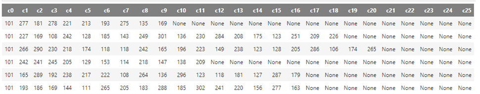
Order data constructed as an ordered sequence of added products
The aggregate function `NTH` is employed to extract the `seq_product_id` from each row in the sequence (where each product added to an order corresponds to a row in the sequence). This ID is then allocated to the appropriate column based on its position within the specific order. This is accomplished by specifying the indices `1` to `25` in the snippet above.
If an order does not contain a product added at a particular position, we encounter a `None` value. These `null` values, in database parlance, must be addressed and cleaned in the subsequent steps.
Final cleaning and persistence of data
At this point, we simply manage the `null` values and add end-of-sentence markers. We’ll leverage Teradata’s robust in-database capabilities to accomplish this.
As a first step, we’ll persist the `prepared_ds` DataFrame to the data warehouse.
prepared_ds.to_sql("prepared_ds", if_exists="replace")
As a next step, we produce a table with the following characteristics:
- We need to insert the final sentence marker `102` after the last product added to each order.
- The value of the columns where no product exists should be `0` instead of `null`.
To meet the specified conditions, we must examine, for each column, whether the column value is `null` and apply conditional modifications based on whether the preceding column contains a product token. If the preceding column does have a product token, the `null` should be replaced with an end-of-sentence marker; otherwise, if it contains another `null` value, it should be replaced with `0`.
The COALESCE function enables us to efficiently apply a condition when the value of a column is `null`. In this context, it is used to inspect each column. If the column’s value is `null`, it checks the preceding column’s value using a CASE statement. The CASE statement allows for conditional logic in SQL. In this situation, if the previous column’s value is `null`, it returns `0`; otherwise, it returns `102`.
We can utilize the following script to preserve a cleaned version that is prepared for the training phase.
create_cleaned_ds_qry = '''

CREATE TABLE cleaned_ds AS (

  SELECT

    c0,

    c1,

    COALESCE(c2, CASE WHEN c1 IS NULL THEN 0 ELSE 102 END) AS c2,

    COALESCE(c3, CASE WHEN c2 IS NULL THEN 0 ELSE 102 END) AS c3,

    COALESCE(c4, CASE WHEN c3 IS NULL THEN 0 ELSE 102 END) AS c4,

    COALESCE(c5, CASE WHEN c4 IS NULL THEN 0 ELSE 102 END) AS c5,

    COALESCE(c6, CASE WHEN c5 IS NULL THEN 0 ELSE 102 END) AS c6,

    COALESCE(c7, CASE WHEN c6 IS NULL THEN 0 ELSE 102 END) AS c7,

    COALESCE(c8, CASE WHEN c7 IS NULL THEN 0 ELSE 102 END) AS c8,

    COALESCE(c9, CASE WHEN c8 IS NULL THEN 0 ELSE 102 END) AS c9,

    COALESCE(c10, CASE WHEN c9 IS NULL THEN 0 ELSE 102 END) AS c10,

    COALESCE(c11, CASE WHEN c10 IS NULL THEN 0 ELSE 102 END) AS c11,

    COALESCE(c12, CASE WHEN c11 IS NULL THEN 0 ELSE 102 END) AS c12,

    COALESCE(c13, CASE WHEN c12 IS NULL THEN 0 ELSE 102 END) AS c13,

    COALESCE(c14, CASE WHEN c13 IS NULL THEN 0 ELSE 102 END) AS c14,

    COALESCE(c15, CASE WHEN c14 IS NULL THEN 0 ELSE 102 END) AS c15,

    COALESCE(c16, CASE WHEN c15 IS NULL THEN 0 ELSE 102 END) AS c16,

    COALESCE(c17, CASE WHEN c16 IS NULL THEN 0 ELSE 102 END) AS c17,

    COALESCE(c18, CASE WHEN c17 IS NULL THEN 0 ELSE 102 END) AS c18,

    COALESCE(c19, CASE WHEN c18 IS NULL THEN 0 ELSE 102 END) AS c19,

    COALESCE(c20, CASE WHEN c19 IS NULL THEN 0 ELSE 102 END) AS c20,

    COALESCE(c21, CASE WHEN c20 IS NULL THEN 0 ELSE 102 END) AS c21,

    COALESCE(c22, CASE WHEN c21 IS NULL THEN 0 ELSE 102 END) AS c22,

    COALESCE(c23, CASE WHEN c22 IS NULL THEN 0 ELSE 102 END) AS c23,

    COALESCE(c24, CASE WHEN c23 IS NULL THEN 0 ELSE 102 END) AS c24,

    CASE WHEN c25 IS NULL THEN 0 ELSE 102 END AS c25

  FROM prepared_ds

) WITH DATA;

'''

tdml.execute_sql(create_cleaned_ds_qry)
- The resulting data would look like this:
cleaned_ds_dtf = tdml.DataFrame('cleaned_ds')

cleaned_ds_dtf
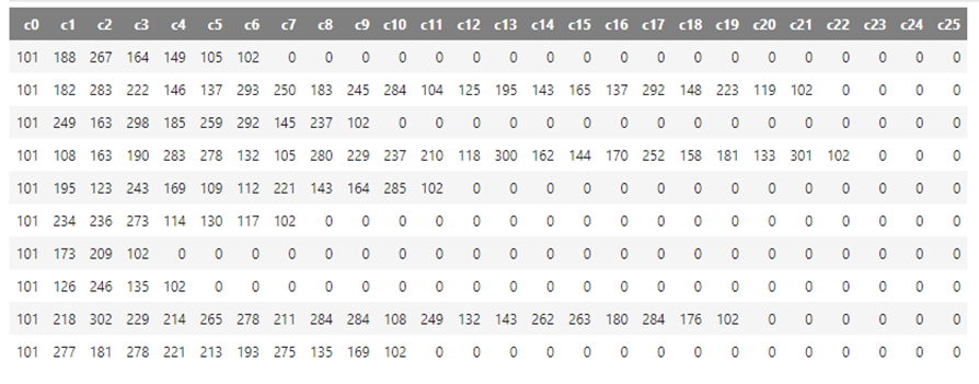
Cleaned product sequence data
The cleaned training dataset can be persisted to object storage for easy consumption by any ML tool on any cloud.
We could easily store the data in a Parquet file within Microsoft Azure, for example, with a simple statement like the one below. Similarly, the data could also be stored to any other object storage provider supported by Teradata’s Native Object Store (NOS).
SELECT NodeId, AmpId, Sequence, ObjectName, ObjectSize, RecordCount

FROM WRITE_NOS_FM (

    ON (

        select * from cleaned_ds

    )

    USING

    LOCATION('/AZ/<azure_blob_storage_folder>/')

    STOREDAS('PARQUET')

    COMPRESSION('GZIP')

    NAMING('RANGE')

    INCLUDE_ORDERING('TRUE')

    MAXOBJECTSIZE('4MB')

) AS d

ORDER BY AmpId;
This command can be run directly in the Jupyter Notebook through the corresponding engine or any database client. The snippet is provided for reference only, since block storage is not provided as part of this walkthrough.
Model training
We’re now prepared to begin training a model. Teradata VantageCloud can easily be integrated with Microsoft Azure Machine Learning, especially if you already have a Teradata VantageCloud Lake instance in the platform. Integration is also very convenient with Amazon SageMaker and Google Cloud Vertex AI.
In the sample we’ve been examining, the data utilized for training is composed of the `orders` data, which is systematically arranged based on the sequential addition of products to each order. During the training phase, the aim is to discern connections between products, with a particular focus on their sequence of addition to the shopping cart. Essentially, we’re attempting to allocate a probability to the event of adding a specific item — for instance, hot dogs — after the inclusion of another item — like bread — in the shopping cart. This is analogous to discovering the order of words in a sentence based on the context.
The vector space in which the products’ "words" are assigned a value based on their relation to each other is called an embedding. The type of neural network used to discover these types of relations is called a transformer.
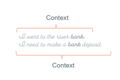
Example of context as related to words in a sentence
Since neural networks discover relationships by masking some values in the sentence and trying to guess what "word" should occupy that space, the process is computationally expensive.
Training in the cloud offers the advantage of scalability and cost-performance, since compute resources can be engaged when they are cheapest, and to the amount that is strictly needed.
During training, the predictive capability of the model is continually tested. For this purpose, usually the available data is divided between a training set, used to train the model, and a testing set. When the predictive capability of the model is deemed good enough, in accordance with the business requirements and business and technical constraints, the model is ready for operationalization.
In our case, once trained, our language model can be utilized to carry out tasks like generating a sequence of products, which can then serve as recommendations for consumers.
Model operationalization
Model deployment
In the past, it was common to build services around the environment on which the model was built. These services usually exposed endpoints to request predictions from the model. Under this type of architecture, the processes needed for maintaining the model (adjustment, training on new results, etc.) and the efficiency of the systems depending on it were not optimal. Maintenance and scalability often required the replication of the deployment environment, and replicating the entirety of an environment is not straightforward. For this reason, standards, such as ONNX, have been developed to export the model configuration easily. It is common practice to export these files to an independent service and build API endpoints around that system. However, this only solves part of the problem, since the model is still isolated from the business context.
Teradata VantageCloud incorporates Bring Your Own Model (BYOM) . BYOM allows importing of the model, as an ONNX file, for example, into the data warehouse or data lake. The model becomes, under this paradigm, another asset in your data environment. Predictions can be made as queries to the data warehouse, or data lake scoring of the model becomes an in-database operation, streamlining the process of model update and refinement.
The deployment of a model in this scenario could be something as simple as the code below, where you identify your model and the table you want to export it to, and voilà!
#deploy downloaded model to Teradata

print(f'Deploying model with id "%s" to table "%s"...' % (deployment_conf["model_id"], deployment_conf['model_table']))

tdml.delete_byom(

    deployment_conf["model_id"],

    deployment_conf['model_table'])

tdml.save_byom(

    deployment_conf["model_id"],

   './' + model_file_path,

    deployment_conf['model_table'])
Predictions are made by querying the deployed model. This can be done through a function like the one below (though the actual query would vary according to the model deployment parameters).
def get_context_based_recommendations(product_names, rec_number = 5, overwrite_cache = False):

    seq_ids = collect_seq_ids(prouct_names)

    select_tensor = generate_select_tensor(seq_ids, 32)
    query = f"""query to the model"""%(

        select_tensor,

       deployment_conf["model_table"],

       deployment_conf["model_id"],

       f"OverwriteCachedModel('%s')"%deployment_conf["model_id"] if overwrite_cache else "",

        rec_number

        )
result = {}
sql_res = conn.execute(query)
    for row in sql_res:

        result[row["num"]] = {"product_name": row["product_name"], "product_id": row["product_id"], "department_id": row["department_id"], "aisle_id": row["aisle_id"]}
return result
Model operations
In the context of our example, we could run very straightforward SQL commands to retrieve recommendations from the model deployed in our data warehouse or data lake. This has the added advantage that the recommendations from the model could be refined with context from other data in our data environment, previous history of the specific customer, local offerings according to the customer location, and many other parameters. This is an advantage that an isolated generative AI model would not be able to integrate.
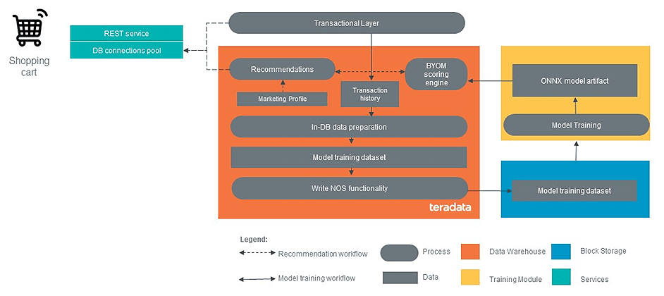
A diagram that depicts the implementation of an end-to-end ML pipeline with Teradata VantageCloud.
Finally, with tools such as ModelOps, we can easily measure the performance of the model and keep tabs on when it should be updated or further refined.
Conclusion
We’ve outlined ClearScape Analytics’ analytical capabilities across the various stages of the ML life cycle. When it comes to the analysis and transformation of data during the problem definition and data preparation stage, ClearScape Analytics’ analytic capabilities are unparalleled. VantageCloud’s robust cloud native offerings enable a seamless transition from operational data to model training on cutting-edge platforms. Finally, tools such as BYOM and ModelOps facilitate immediate deployment, operationalization, and monitoring of models, not in isolation, but within the business context where these models are designed to add value.
Feedback & questions
We value your insights and perspective! Share your thoughts, feedback, and ideas in the comments below. Feel free to explore the wealth of resources available on the Teradata Developer Portal and Teradata Developer Community.
最新情報をお受け取りください
メールアドレスをご登録ください。ブログの最新情報をお届けします。